Linear map

In mathematics, a linear map (also called a linear transformation, linear function or linear operator) is a function between two vector spaces that preserves the operations of vector addition and scalar multiplication. The expression "linear operator" is commonly used for linear maps from a vector space to itself (endomorphisms). In advanced mathematics, the definition of linear function coincides with the definition of linear map.

In the language of abstract algebra, a linear map is a homomorphism of vector spaces, or in the language of category theory a morphism in K-Vect, the category of vector spaces over a given field K.

1 Definition and first consequences
2 Examples
3 Matrices
4 Examples of linear transformation matrices
5 Forming new linear maps from given ones
6 Endomorphisms and automorphisms
7 Kernel, image and the rank-nullity theorem
8 Cokernel
- 8.1 Index
9 Algebraic classifications of linear transformations
10 Continuity
11 Applications
12 See also
13 References

Definition and first consequences

Let V and W be vector spaces over the same field K. A function f : V → W is said to be a linear map if for any two vectors x and y in V and any scalar a in K, the following two conditions are satisfied:

$f(x+y)=f(x)+f(y) \,$	additivity
$f(ax)=af(x) \,$	homogeneity of degree 1.

This is equivalent to requiring that for any vectors x₁, ..., x_m and scalars a₁, ..., a_m, the equality

$f(a_1 x_1+\cdots+a_m x_m)=a_1 f(x_1)+\cdots+a_m f(x_m)$

holds.

It immediately follows from the definition that f(0) = 0.

Occasionally, V and W can be considered to be vector spaces over different fields. It is then necessary to specify which of these ground fields is being used in the definition of "linear". If V and W are considered as spaces over the field K as above, we talk about K-linear maps. For example, the conjugation of complex numbers is an R-linear map C → C, but it is not C-linear.

A linear map from V to K (with K viewed as a vector space over itself) is called a linear functional.

Examples

The identity map and zero map are linear.
The map $x\mapsto cx$ , where c is a constant, is linear.
For real numbers, the map $x\mapsto x^2$ is not linear.
For real numbers, the map $x\mapsto x+1$ is not linear (but is an affine transformation, and also a linear function.)
If A is a real m × n matrix, then A defines a linear map from Rⁿ to R^m by sending the column vector x ∈ Rⁿ to the column vector Ax ∈ R^m. Conversely, any linear map between finite-dimensional vector spaces can be represented in this manner; see the following section.
The integral is a linear map from the space of all real-valued integrable functions on some interval to R
Differentiation is a linear map from the space of all differentiable functions to the space of all functions.
If V and W are finite-dimensional vector spaces over a field F, then functions that send linear maps f : V → W to dim_F(W)-by-dim_F(V) matrices in the way described in the sequel are themselves linear maps.
The expected value of a random variable X is linear, as $E[cX + a] = cE[X] + a$ , but the variance of a random variable is not linear, as it violates the second condition, homogeneity of degree 1: $V[cX + a] = c^2V[X]$ .

Matrices

If V and W are finite-dimensional, and one has chosen bases in those spaces, then every linear map from V to W can be represented as a matrix; this is useful because it allows concrete calculations. Conversely, matrices yield examples of linear maps: if A is a real m-by-n matrix, then the rule f(x) = Ax describes a linear map Rⁿ → R^m (see Euclidean space).

Let $\{v_1, \cdots, v_n\}$ be a basis for V. Then every vector v in V is uniquely determined by the coefficients $c_1, \cdots, c_n$ in

$c_1 v_1+\cdots+c_n v_n.$

If f : V → W is a linear map,

$f(c_1 v_1+\cdots+c_n v_n)=c_1 f(v_1)+\cdots+c_n f(v_n),$

which implies that the function f is entirely determined by the values of 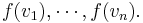$f(v_1),\cdots,f(v_n).$

Now let $\{w_1, \dots, w_m\}$ be a basis for W. Then we can represent the values of each $f(v_j)$ as

$f(v_j)=a_{1j} w_1 + \cdots + a_{mj} w_m.$

Thus, the function f is entirely determined by the values of $a_{i,j}.$

If we put these values into an m-by-n matrix M, then we can conveniently use it to compute the value of f for any vector in V. For if we place the values of $c_1, \cdots, c_n$ in an n-by-1 matrix C, we have MC = the m-by-1 matrix whose i.th element is the coordinate of f(v) which belongs to the base $w_i$ .

A single linear map may be represented by many matrices. This is because the values of the elements of the matrix depend on the bases that are chosen.

Examples of linear transformation matrices

Some special cases of linear transformations of two-dimensional space R² are illuminating:

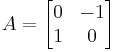
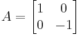
rotation by 90 degrees counterclockwise:

$A=\begin{bmatrix}0 & -1\\ 1 & 0\end{bmatrix}$
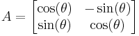
rotation by θ degrees counterclockwise:

$A=\begin{bmatrix}\cos(\theta) & -\sin(\theta)\\ \sin(\theta) & \cos(\theta)\end{bmatrix}$
reflection against the x axis:

$A=\begin{bmatrix}1 & 0\\ 0 & -1\end{bmatrix}$
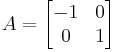
reflection against the y axis:

$A=\begin{bmatrix}-1 & 0\\ 0 & 1\end{bmatrix}$
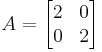
scaling by 2 in all directions:

$A=\begin{bmatrix}2 & 0\\ 0 & 2\end{bmatrix}$
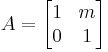
horizontal shear mapping:

$A=\begin{bmatrix}1 & m\\ 0 & 1\end{bmatrix}$
squeezing:

$A=\begin{bmatrix}k & 0\\ 0 & 1/k\end{bmatrix}$
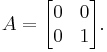
projection onto the y axis:

$A=\begin{bmatrix}0 & 0\\ 0 & 1\end{bmatrix}.$

Forming new linear maps from given ones

The composition of linear maps is linear: if f : V → W and g : W → Z are linear, then so is their composition g o f : V → Z. It follows from this that the class of all vector spaces over a given field K, together with K-linear maps as morphisms, forms a category.

The inverse of a linear map, when defined, is again a linear map.

If f₁ : V → W and f₂ : V → W are linear, then so is their sum f₁ + f₂ (which is defined by (f₁ + f₂)(x) = f₁(x) + f₂(x)).

If f : V → W is linear and a is an element of the ground field K, then the map af, defined by (af)(x) = a (f(x)), is also linear.

Thus the set L(V,W) of linear maps from V to W itself forms a vector space over K, sometimes denoted Hom(V,W). Furthermore, in the case that V=W, this vector space (denoted End(V)) is an associative algebra under composition of maps, since the composition of two linear maps is again a linear map, and the composition of maps is always associative. This case is discussed in more detail below.

Given again the finite-dimensional case, if bases have been chosen, then the composition of linear maps corresponds to the matrix multiplication, the addition of linear maps corresponds to the matrix addition, and the multiplication of linear maps with scalars corresponds to the multiplication of matrices with scalars.

Endomorphisms and automorphisms

A linear transformation f : V → V is an endomorphism of V; the set of all such endomorphisms End(V) together with addition, composition and scalar multiplication as defined above forms an associative algebra with identity element over the field K (and in particular a ring). The multiplicative identity element of this algebra is the identity map id : V → V.

An endomorphism of V that is also an isomorphism is called an automorphism of V. The composition of two automorphisms is again an automorphism, and the set of all automorphisms of V forms a group, the automorphism group of V which is denoted by Aut(V) or GL(V). Since the automorphisms are precisely those endomorphisms which possess inverses under composition, Aut(V) is the group of units in the ring End(V).

If V has finite dimension n, then End(V) is isomorphic to the associative algebra of all n by n matrices with entries in K. The automorphism group of V is isomorphic to the general linear group GL(n, K) of all n by n invertible matrices with entries in K.

Kernel, image and the rank-nullity theorem

If f : V → W is linear, we define the kernel and the image or range of f by

$\operatorname{\ker}(f)=\{\,x\in V:f(x)=0\,\}$

$\operatorname{im}(f)=\{\,w\in W:w=f(x),x\in V\,\}$

ker(f) is a subspace of V and im(f) is a subspace of W. The following dimension formula, known as the rank-nullity theorem, is often useful:

$\dim(\ker( f )) + \dim(\operatorname{im}( f )) = \dim( V ). \,$

The number dim(im(f)) is also called the rank of f and written as rank(f), or sometimes, ρ(f); the number dim(ker(f)) is called the nullity of f and written as null(f) or ν(f). If V and W are finite-dimensional, bases have been chosen and f is represented by the matrix A, then the rank and nullity of f are equal to the rank and nullity of the matrix A, respectively.

Cokernel

A subtler invariant of a linear transformation is the cokernel, which is defined as

$\mathrm{coker}\,f�:= W/f(V) = W/\mathrm{im}(f).$

This is the dual notion to the kernel: just as the kernel is a subspace of the domain, the co-kernel is a quotient space of the target. Formally, one has the exact sequence

$0 \to \ker f \to V \to W \to \mathrm{coker}\,f \to 0.$

These can be interpreted thus: given a linear equation $f(v)=w$ to solve,

the kernel is the space of solutions to the homogeneous equation $f(v)=0,$ and its dimension is the number of degrees of freedom in a solution, if it exists;
the co-kernel is the space of constraints that must be satisfied if the equation is to have a solution, and its dimension is the number of constraints that must be satisfied for the equation to have a solution.

The dimension of the co-kernel and the dimension of the image (the rank) add up to the dimension of the target space. For finite dimensions, this means that the dimension of the quotient space $W/f(V)$ is the dimension of the target space minus the dimension of the image.

As a simple example, consider the map $f\colon \mathbf{R}^2 \to \mathbf{R}^2,$ given by $f(x,y) = (0,y).$ Then for an equation $f(x,y)=(a,b)$ to have a solution, we must have $a=0$ (one constraint), and in that case the solution space is $(x,b),$ or equivalently stated, $(0,b)+(x,0),$ (one degree of freedom). The kernel may be expressed as the subspace $(x,0) < V:$ the value of x is the freedom in a solution – while the cokernel may be expressed via the map $W \to \mathbf{R}^1, (a,b) \mapsto (a):$ given a vector $(a,b),$ the value of a is the obstruction to there being a solution.

An example illustrating the infinite-dimensional case is afforded by the map $g\colon \mathbf{R}^\infty \to \mathbf{R}^\infty, \{a_n\} \to \{b_n\}$ with $b_1 = 0$ and $b_{n+1} = a_n$ for $n > 0$ . Its image consists of all sequences with first element 0, and thus its cokernel consists of the classes of sequences with identical first element. Thus, whereas its kernel has dimension 0 (it maps only the zero sequence to the zero sequence), its co-kernel has dimension 1. Since the domain and the target space are the same, the rank and the dimension of the kernel add up to the same sum as the rank and the dimension of the co-kernel ( $\aleph_0 + 0 = \aleph_0 + 1$ ), but in the infinite-dimensional case it cannot be inferred that the kernel and the co-kernel of an endomorphism have the same dimension ( $0 \neq 1$ ). The reverse situation obtains for the map $h\colon \mathbf{R}^\infty \to \mathbf{R}^\infty, \{a_n\} \to \{c_n\}$ with $c_n = a_{n+1}$ . Its image is the entire target space, and hence its co-kernel has dimension 0, but since it maps all sequences in which only the first element is non-zero to the zero sequence, its kernel has dimension 1.

Index

For a linear operator with finite-dimensional kernel and co-kernel, one may define index as:

$\mathrm{ind}\,f�:= \dim \ker f - \dim \mathrm{coker}\,f,$

namely the degrees of freedom minus the number of constraints.

For a transformation between finite-dimensional vector spaces, this is just the difference $\dim V - \dim W,$ by rank-nullity. This gives an indication of how many solutions or how many constraints one has: if mapping from a larger space to a smaller one, the map may be onto, and thus will have degrees of freedom even without constraints. Conversely, if mapping from a smaller space to a larger one, the map cannot be onto, and thus one will have constraints even without degrees of freedom.

The index comes of its own in infinite dimensions: it is how homology is defined, which is a central theory in algebra and algebraic topology; the index of an operator is precisely the Euler characteristic of the 2-term complex $0 \to V \to W \to 0.$ In operator theory, the index of Fredholm operators is an object of study, with a major result being the Atiyah–Singer index theorem.

Algebraic classifications of linear transformations

No classification of linear maps could hope to be exhaustive. The following incomplete list enumerates some important classifications that do not require any additional structure on the vector space.

Let V and W denote vector spaces over a field, F. Let T:V → W be a linear map.

T is said to be injective or a monomorphism if any of the following equivalent conditions are true:
- T is one-to-one as a map of sets.
- kerT = 0_V
- T is monic or left-cancellable, which is to say, for any vector space U and any pair of linear maps R:U → V and S:U → V, the equation TR=TS implies R=S.
- T is left-invertible, which is to say there exists a linear map S:W → V such that ST is the identity map on V.

T is said to be surjective or an epimorphism if any of the following equivalent conditions are true:
- T is onto as a map of sets.
- coker T = 0
- T is epic or right-cancellable, which is to say, for any vector space U and any pair of linear maps R:W → U and S:W → U, the equation RT=ST implies R=S.
- T is right-invertible, which is to say there exists a linear map S:W → V such that TS is the identity map on V.

T is said to be an isomorphism if it is both left- and right-invertible. This is equivalent to T being both one-to-one and onto (a bijection of sets) or also to T being both epic and monic, and so being a bimorphism.

If T: V → V is an endomorphism, then:
- If, for some positive integer n, the n-th iterate of T, Tⁿ, is identically zero, then T is said to be nilpotent.
- If T T = T, then T is said to be idempotent
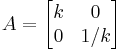
- If T = k I, where k is some scalar, then T is said to be a scaling transformation or scalar multiplication map; see scalar matrix.

Continuity

A linear operator between topological vector spaces, for example normed spaces, may also be continuous and therefore be a continuous linear operator. On a normed space, a linear operator is continuous if and only if it is bounded, for example, when the domain is finite-dimensional. If the domain is infinite-dimensional, then there may be discontinuous linear operators. An example of an unbounded, hence not continuous, linear transformation is differentiation on the space of smooth functions equipped with the supremum norm (a function with small values can have a derivative with large values, while the derivative of 0 is 0).

Applications

A specific application of linear maps is for geometric transformations, such as those performed in computer graphics, where the translation, rotation and scaling of 2D or 3D objects is performed by the use of a transformation matrix.

Another application of these transformations is in compiler optimizations of nested-loop code, and in parallelizing compiler techniques.

References

Halmos, Paul R. (1974), Finite-dimensional vector spaces, New York: Springer-Verlag, ISBN 978-0-387-90093-3
Lang, Serge (1987), Linear algebra, New York: Springer-Verlag, ISBN 978-0-387-96412-6

Topics related to linear algebra

Scalar · Vector · Vector space · Vector projection · Linear span · Linear map · Linear projection · Linear independence · Linear combination · Basis · Column space · Row space · Dual space · Orthogonality · Rank · Minor · Kernel (matrix) · Eigenvalue, eigenvector and eigenspace · Least squares regressions · Outer product · Inner product space · Dot product · Transpose · Gram–Schmidt process · Matrix decomposition